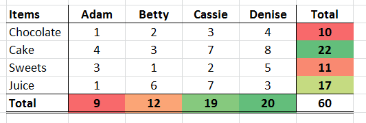
Conditional
Formatting
This is a
very useful trick if you have to analyze huge bunch of numbers all the time.
Imagine you have a very big table and you are trying to figure out the trend or
trying to find the largest number. The quickest and most intuitional way of
doing this is by using conditional formatting.
It is an
in-built function in Excel that allows you capturing any trend/pattern in the
data within seconds.
Now, go to “Home” ribbon, and click on “Conditional
Formatting”. Then, go to “Colour Scales” and choose your favourite colour
scales to apply on the data.

As our intention is to introduce you “Conditional Formatting”, we will leave you to explore on other potential usage of this amazing function. As you can see, there are still plenty of options that can be chosen from.
I assure you that each of them is very helpful and worth your time exploring.
Proceed to next awesome trick: Excel Level-Up: Day 8
No comments:
Post a Comment